Classical Recommendation-System Techniques - A Quick Overview

TL;DR — From TikTok’s ‘For You’ feed to your favourite delivery app, recommender systems decide what you see next. This post walks absolute beginners through six classical techniques—no PhD jargon, just intuitive visuals and a single running example.

Here the video to it:

Meet our running example

You own a small restaurant that takes online orders. You want to suggest dishes your customers will probably love. Throughout the post we’ll reuse the same tiny data set:

Dish	Tags
Shawarma	spicy, chicken
Burger	beef, hearty
Milkshake	sweet, vanilla‑or‑chocolate
Fries	side‑dish, potato

Our historical orders look like this (1 = ordered):

User	Shawarma (D1)	Burger (D2)	Milkshake (D3)	Fries (D4)
Ahmed	1	0	1	0
Fatima	0	0	1	1
Bilal	1	1	0	0

1. Memory‑based Collaborative Filtering – “Customers that behave alike”

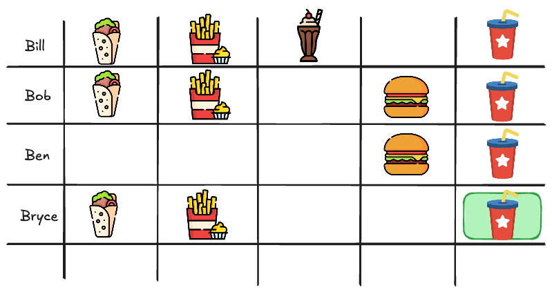
To start recommending dishes, you first want to see what your customers even like. So you decide to make a list of all the dishes that your customers have ordered in the past.

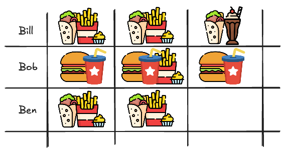
Bill has recently tried the combination of the Shawarma with the Milkshake and loved it. You see that in the past Ben has ordered the same dishes as Bill and so you decide to recommend the Shawarma and Milkshake to Ben. This is called Memory-based Collaborative Filtering. It works by finding customers that behave alike and recommending items that they have liked in the past.

These types of Recommendations are great for tiny data sets, however they become noisy as the menu or customer base grows.

2. Matrix Factorization

You now want to explore exatly how and why people like dishes.

For example:

• Some customers like spicy and low-calorie foods.
• Others like meaty and very heavy foods.

Let's say again these are the dishes you have:

Dish	Description
Shawarma	Spicy, Chicken
Burger	Not spicy, Beef
Milkshake	Sweet, Vanilla or Chocolate
Fries	Not spicy, Potato, Side dish

Imagine you have a customer called Ahmed. You don't know Ahmed personally, but you know he liked the Shawarma and the milkshake. You want to predict if Ahmed would like the Burger or Fries next.

But here's the thing: Matrix Factorization doesn't look at the dish description directly (like "spicy" or "beef"). Instead, it says:

"Let’s learn a hidden profile for Ahmed based on what he liked, and a hidden profile for each dish, and see which ones match"

Customer	Shawarma	Burger	Milkshake	Fries
Ahmed	1	?	1	?

We then create a matrix of all the dishes and their hidden profiles. For example:

Dish	Spice	Sweetness
Shawarma	0.9	0.1
Burger	0.2	0.1
Milkshake	0.0	1.0
Fries	0.1	0.0

We can then Plot them in a 2D space as such:

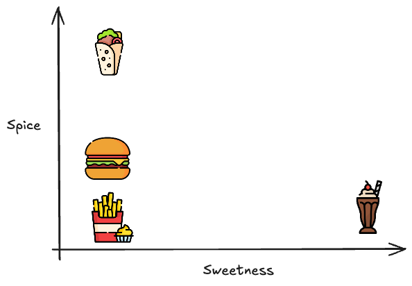
We now do a “matching score” between Ahmed and each dish by multiplying these hidden features.

Since Ahmed liked the Shawarma and Milkshake, the score could look like this, it could be that Ahmed likes 0.8 spicy and 0.5 sweet.

We then compare the scores of the dishes with the scores of Ahmed:

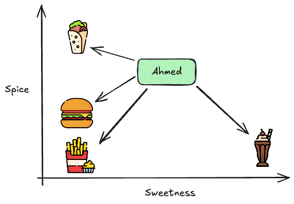
Finding the clossest analytically is done using the dot product of Ahmed to the dishes:

$$\text{Score} = \vec{u}{Ahmed} \cdot \vec{v}{Dish} = (a_1 \times d_1) + (a_2 \times d_2)$$

e.g. For the Shawarma:

$$\text{Score} = (0.8 \cdot 0.9) + (0.5 \cdot 0.1) = 0.72 + 0.05 = \boxed{0.77}$$

And for the others:

• Burger: 0.21
• Milkshake: 0.58
• Fries: 0.08

And so we recommend the Shawarma to Ahmed again.

But Where do those hidden numbers like 0.8 for ‘spicy’ come from? I didn’t define them anywhere? We kinda left this big part out.

And the short answer is:

• You don’t manually define those values.
• Matrix Factorization learns them automatically during training.

The long answer is the following:

Let’s say you have just an order history, like this:

User	Shawarma (D1)	Burger (D2)	Milkshake (D3)	Fries (D4)
Ahmed	1	0	1	0
Fatima	0	0	1	1
Bilal	1	1	0	0

We want to learn:

A taste vector for each user (Ahmed, Fatima, Bilal)

A feature vector for each dish (D1, D2, D3, D4)

So that:

$$\text{Predicted Score} = \text{dot product of (User Vector, Dish Vector)}$$

is close to 1 if ordered, 0 if not ordered.

Be do this with the following steps:

1: Initialize random vectors

User	Feature 1	Feature 2
Ahmed	0.6	0.3
Fatima	0.2	0.8
Bilal	0.7	0.2

Dish	Feature 1	Feature 2
Shawarma	0.8	0.1
Burger	0.6	0.2
Milkshake	0.1	0.9
Fries	0.2	0.8

2: Predict scores with dot products

e.g. For Ahmed and Shawarma:

$$(0.6 × 0.8) + (0.3 × 0.1) = 0.48 + 0.03 = 0.51$$

Here all the scores:

User	Shawarma	Burger	Milkshake	Fries
Ahmed	0.51	0.42	0.33	0.36
Fatima	0.24	0.28	0.74	0.68
Bilal	0.58	0.46	0.25	0.30

3: Check error

These are of course not the right scores. We want to minimize the error between the predicted scores and the actual scores.

User	Dish	True	Predicted	Error
Ahmed	Shawarma	1	0.51	High error
Ahmed	Burger	0	0.42	High error
Ahmed	Milkshake	1	0.33	High error
Ahmed	Fries	0	0.36	High error

And do this with the entire matrix.

4: Update vectors

What the algorithm would now do:

• See that Ahmed's score for Shawarma (0.51) is too low for a real order → increase similarity between Ahmed and Shawarma.
• See that Ahmed's score for Burger (0.42) is too high for a non-order → decrease similarity between Ahmed and Burger.

It would update the vectors:

• Slightly move Ahmed's vector closer to Shawarma’s vector.
• Slightly move Ahmed's vector away from Burger’s vector.
• Slightly move Milkshake’s vector closer to Ahmed, and so on...

Over many small updates, the vectors become better aligned with the true orders.

This is done using a technique called Stochastic Gradient Descent (SGD). It’s a way to adjust the vectors in small steps to minimize the error.

In python we would do the following:

3. Neural Collaborative Filtering

Now this builds a bit on top of the matrix factorization. It uses a neural network to learn the hidden features of the users and dishes.

Here a couple of differences:

Matrix Factorization	Neural Collaborative Filtering
Matches user and item with dot-product (linear math)	Matches user and item with a tiny neural network (non-linear math)
Only captures straight-line relationships	Captures complex, messy relationships
Easy but limited	Harder but smarter

Example:

• MF can say "Ahmed likes spicy dishes."
• NCF can say "Ahmed likes spicy dishes only if they are low-calorie." (because neural networks can model AND, OR, IF-THEN rules)

This is how we would do it:

1: Create Embeddings

This is the same as in matrix factorization. We create a vector for each user and each dish.

User	Feature 1	Feature 2
Ahmed	0.6	0.3
Fatima	0.2	0.8
Bilal	0.7	0.2

Dish	Feature 1	Feature 2
Shawarma	0.8	0.1
Burger	0.6	0.2
Milkshake	0.1	0.9
Fries	0.2	0.8

These are randomly initialized at first and learned over time.

2: Combine User and Item Embeddings

Instead of doing dot-product like MF, NCF Concatenates user and item vectors into one big vector.

Example for Ahmed and Shawarma:

$$[0.8, 0.5] + [0.9, 0.2] = [0.8, 0.5, 0.9, 0.2]$$

3: Feed into a small Neural Network

Now we need to create the Neural Network architecture. This looks hihghly complex, but it’s actually quite simple. You can watch StatQuest’s video on Neural Networks. I don't think I could explain it better than him.

But this is how the Architecture would look like, it's just a Multi-Layer Perceptron = MLP:

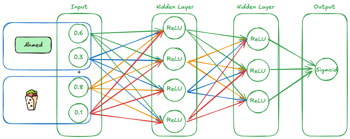
Each neuron applies:

• A weighted sum of inputs
• A non-linear activation (like ReLU or Sigmoid)

Then we just need to train the network using backpropagation. This is a way to adjust the weights of the neurons based on the error between the predicted and actual scores and then we're done.

4. Content‑based Filtering

Imagine here the following table of dishes:

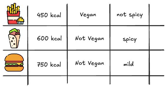
This works by making each dish a vector based on its attributes. The system then compares the vectors of the dishes to find the best match for the customer’s preferences.

To compare the vectors, you can use cosine similarity. This is a measure of how similar two vectors are. The closer the cosine similarity is to 1, the more similar the vectors are.

$$\text{cosine\_similarity} = \frac{A \cdot B}{\|A\| \cdot \|B\|}$$

Where (A) is the seach vector and (B) is the dish.

This gives a similarity score between -1 and 1, where:

• 1 = perfect match in direction
• 0 = no directional similarity
• -1 = exactly opposite direction

For the Search vector $(500, 1, 0)$:

$$\|Search\| = \sqrt{500^2 + 1^2 + 0^2} = \sqrt{250000 + 1} = \sqrt{250001} \approx 500.001$$

We can then calculate the Cosine similariy as such for the Fries: (450, 1, 0):

Dot product:

$$(500 \cdot 450) + (1 \cdot 1) + (0 \cdot 0) = 225001$$

Magnitude:

$$\sqrt{450^2 + 1^2 + 0^2} = \sqrt{202500 + 1} = \sqrt{202501} \approx 449.999$$

Cosine similarity:

$$\frac{225001}{500.001 \cdot 449.999} \approx \frac{225001}{225000.45} \approx \boxed{1.0000}$$

The results for the other dishes are:

Burger: 0.999998 and Shawarma: 0.999997

This means that the search vector and the fries vector are the most similar, and the system will recommend the fries to the customer.

These Systems are great for Cold-start customers where you dont have any past explanations yet, and they are fully explainable. However, they rely on good human‑made tags, and so might not be too useful for overly complex systems where the tags are not so clear. This could be changed in the future with LLMs tagging complex data.

5. Sequential models

If a user’s current cart is Chicken Shawarma + Fries, sequential models treat that as a sequence and try to predict the next addition to the cart. Often the answer might be "Soft Drink" and so the user get's recommended that.

These systems are great for capturing context & bundle logic, but they have a hard time with new items where there is no sequence yet. You can think of this as similar to new Youtube videos that have no views yet. The Algorithm has no idea with what to recommend them with and who the target audience is.

6. Graph‑based models

Lastly we have Graph-based models. These are great for capturing complex relationships between users and items.

Instead of looking at users and items separately, Graph models treat the entire system as a network of users and items connected by interactions.

• Every user and every item is a node.
• Every purchase is a connection (edge) between them.

Then, we spread signals across this graph to recommend new items.

This could look something like this:

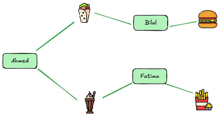
We can now spread information across the graph to find similar users and items. We can see here for instance that both Ahmed and Fatima are connected to the Milkshake. However Fatima is also connected to the Fries. So we can recommend the Fries to Ahmed as well.

These models are powerful because they can capture complex relationships between users and items, especially in communities.