"Computer Science is no more about computers than astronomy is about telescopes." - Edsger W. Dijkstra

ok, let's get something out of the way: I'm not a math teacher, I'm still working on my degree and I'm not particularly good at math... But why am I then creating a full on lesson on Matrices? Really for a selfish reason:

To learn it better myself

Honestly, teaching is one of the best ways to actually learn something deeply. I've got exams coming up, and explaining these concepts makes them click for me in a way that just cramming never could. Plus, I'm naturally curious, and turning my study notes into something teachable keeps that curiosity alive.

Math used to feel like a constant struggle. I'd always be asking myself questions like "Why do I even need this?" or "How will this ever help me in the real world?" I'm pretty sure I'm not the only one who's felt that way. So here's my goal: to explain this stuff in a way that actually makes sense and feels useful.

Along the way, I've learned how to use tools like NumPy, Pandas, and PyTorch more effectively, and I've even picked up some basics of computer graphics. Pretty cool for something I used to avoid, right?

While having created this script, I got a deep appreciation for math. Something I've never felt before. I hope in a way I can now share this with anyone reading this. Know that there is a reason for this struggle, and that it is worth it.

I wrote this script in a way I would have liked to have been taught this topic. This is basically me teaching myself the topics and finding cool ways to apply them. I hope this helps you as it helped me.

Matrices might sound fancy, but they're really just arrays of arrays—a concept most of us programmers are already familiar with. Here's an example in JavaScript:

const matrix = [[1, 2, 3],[1, 2, 3],[1, 2, 3]]

In a way, it is just another data structure with deep roots in mathematics. It's biggest use cases as far as I see it in Software is:

• A way to define and manipulate images
• A way to define and manipulate Datasets

Meaning, they are used a lot in Computer graphics, Data Science and Machine learning. In fact, Machine learning is kinda just Linear algebra to begin with, and understanding Matrices to a deep degree would allow you to grasp Machine learning algorithms a lot better.

You can see them as a necessary building block to Machine Learning.

Think of matrices as the building blocks of everything from AI to image processing. Once you get comfortable with them, you'll start seeing them everywhere.

Side Note: If you're a web developer, you might never need linear algebra in your job. I didn't for years. But if you love learning and want to level up your skills, understanding matrices can give you a new appreciation for the tools and systems we use daily.

Images as Matrices

As you may remember, Images are made up of many pixels, which all have a value for the color. In a grayscale image, this might look like this:

$$\begin{bmatrix} 120 & 130 & 140 \\ 200 & 210 & 220 \\ 255 & 245 & 235 \end{bmatrix}$$

Grayscale image values go from 0 to 255, where 0 is black and 255 is white. Basically saying how black and white this is.

In contrast, RGB Images have 3 channels, which we can think of as 3 distinct matrices per image, meaning they have 3 times more data in them too.

For a small $2 \times 2$ RGB image:

$$\text{R} = \begin{bmatrix} 255 & 128 \\ 64 & 0 \end{bmatrix}, \quad \text{G} = \begin{bmatrix} 0 & 64 \\ 128 & 255 \end{bmatrix}, \quad \text{B} = \begin{bmatrix} 128 & 255 \\ 64 & 0 \end{bmatrix}$$

The combined RGB image is:

$$\begin{bmatrix} \begin{bmatrix} 255 & 128 \\ 64 & 0 \end{bmatrix}, \begin{bmatrix} 0 & 64 \\ 128 & 255 \end{bmatrix}, \begin{bmatrix} 128 & 255 \\ 64 & 0 \end{bmatrix} \end{bmatrix}$$

Why Does This Matter?

Because manipulating these matrices lets us do amazing things with images, like flipping, rotating, or applying filters. It's the foundation of how image editing software works.

Datasets as Matrices

If we had tabular data as a Dataset, we can represent it as a matrix, using the Features and Labels.

Imagine you had a small dataset, aiming to find the correlation between Hours studied, Breaks taken and the final score you get at an exam.

Hours Studied	Breaks taken	Exam Score
2	3	50
5	1	80
3	2	65

We can Separate this into the Feature Matrix and the Target Vector. Both of these are used a lot in Supervised Machine learning, and I wish I would have learned how matrices are used like this sooner.

• Feature Matrix $\mathbf{X}$ (What we use to make predictions):

$$\mathbf{X} = \begin{bmatrix} 2 & 3 \\ 5 & 1 \\ 3 & 2 \end{bmatrix}$$

• Target Vector $\mathbf{y}$ (What we want to predict):

$$\mathbf{y} = \begin{bmatrix} 50 \\ 80 \\ 65 \end{bmatrix}$$

A linear regression model might predict the exam score using the relationship:

$$\mathbf{y} = \mathbf{X} \cdot \mathbf{w} + \mathbf{b}$$

Where $\mathbf{w}$ (weights) and $\mathbf{b}$ (bias) are learned from the data.

However before we go into how we could solve this example, let us first learn more about Matrices.

Types of Matrices

Matrices come in all shapes and sizes, and we categorize them based on their structure and elements. Let's break it down:

1. Based on Size and Shape

Square Matrix: A matrix with the same number of rows and columns ( $n \times n$ ).

$$A = \begin{bmatrix} 1 & 2 & 3 \\ 4 & 5 & 6 \\ 7 & 8 & 9 \end{bmatrix}$$

Row Matrix: A matrix with a single row ( 1 \times n ).

$$A = \begin{bmatrix} 1 & 2 & 3 \end{bmatrix}$$

Column Matrix: A matrix with a single column ( m \times 1 ).

$$A = \begin{bmatrix} 1 \\ 2 \\ 3 \end{bmatrix}$$

2. Based on Elements

Identity Matrix: A diagonal matrix with all diagonal elements equal to 1.

$$I = \begin{bmatrix} 1 & 0 & 0 \\ 0 & 1 & 0 \\ 0 & 0 & 1 \end{bmatrix}$$

Zero Matrix (Null Matrix): A matrix where all elements are 0.

$$A = \begin{bmatrix} 0 & 0 & 0 \\ 0 & 0 & 0 \end{bmatrix}$$

Upper Triangular Matrix: A square matrix where all elements below the diagonal are 0.

$$A = \begin{bmatrix} 1 & 2 & 3 \\ 0 & 4 & 5 \\ 0 & 0 & 6 \end{bmatrix}$$

Lower Triangular Matrix: A square matrix where all elements above the diagonal are 0.

$$A = \begin{bmatrix} 1 & 0 & 0 \\ 2 & 3 & 0 \\ 4 & 5 & 6 \end{bmatrix}$$

Matrix Operations

Operations, such as Addition and multiplication work a bit differently on Matrices. In this Section we will explore all kinds of Matrix operations through images.

Let us first go through how we will display these operations throughout this section.

Using Python

For this section we will use numpy for Matrix operations and matplotlib to show them. I made a small helper function to display the Matrices as images called show_matrix:

def show_matrix(matrix: np.ndarray, max_value: int = 255):
    plt.imshow(matrix, cmap="gray", vmin=0, vmax=max_value)
    plt.colorbar()
    plt.show()

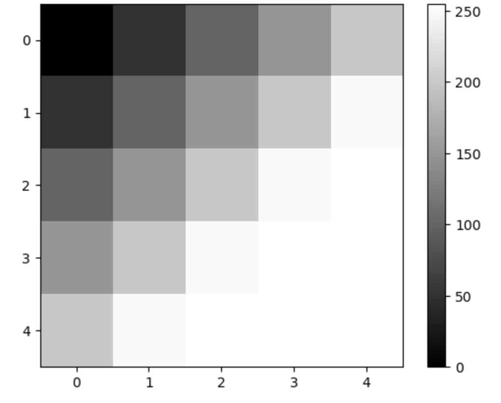
If we were to put in a Grayscale matrix as such:

image = np.array([
    [0, 50, 100, 150, 200],
    [50, 100, 150, 200, 250],
    [100, 150, 200, 250, 255],
    [150, 200, 250, 255, 255],
    [200, 250, 255, 255, 255]
])

show_matrix(image)

We get the following Matrix with it:

Now that this is clear, let's start with the operations

Scalar Multiplication

This is by far the simplest of the Operations. Scalar multiplication involves multiplying each element of a matrix by a scalar (a single number).

$\text{If } A = \begin{bmatrix} 1 & 2 \\ 3 & 4 \end{bmatrix} \text{ and scalar } c = 3, \text{ then } cA = \begin{bmatrix} 3 & 6 \\ 9 & 12 \end{bmatrix}.$

Easy right? Let's move on.

Addition

Matrix addition involves adding the corresponding elements of two matrices. To add two matrices both matrices must have the same dimensions. This is important, it won't work otherwise.

For:

$A = \begin{bmatrix} 1 & 2 \\ 3 & 4 \end{bmatrix}, \quad B = \begin{bmatrix} 5 & 6 \\ 7 & 8 \end{bmatrix}$ The addition would be as such:

$A + B = \begin{bmatrix} 1+5 & 2+6 \\ 3+7 & 4+8 \end{bmatrix} = \begin{bmatrix} 6 & 8 \\ 10 & 12 \end{bmatrix}$

Dot product

The dot product (matrix multiplication) involves multiplying rows of the first matrix with columns of the second matrix and summing the products.

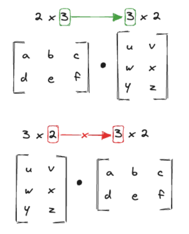
To perform the dot product:

1. The number of columns in the first matrix must match the number of rows in the second matrix.
2. The result is a new matrix where Each element is the sum of the element-wise product of a row from the first matrix and a column from the second matrix.

This is a bit tricky and not that intuitive. The video from 3b1b really helped in showing this.

Let $A$ be a $2 \times 3$ matrix, and $B$ be a $3 \times 2$ matrix:

$$A = \begin{bmatrix} 1 & 2 & 3 \\ 4 & 5 & 6 \end{bmatrix}, \quad B = \begin{bmatrix} 7 & 8 \\ 9 & 10 \\ 11 & 12 \end{bmatrix}$$

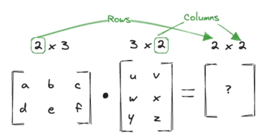
The resulting matrix $C$ will have dimensions $2 \times 2$ because:

$\text{Number of rows in } A = 2, \quad \text{Number of columns in } B = 2$

Calculation of $C = A \cdot B$

Each element $C[i,j]$ is computed as:

$C[i,j] = \sum_k A[i,k] \cdot B[k,j]$

$$C = \begin{bmatrix} 58 & 64 \\ 139 & 154 \end{bmatrix}$$

What's important here, is that the number of columns of the first Matrix must equal the rows of the second matrix.

The Dimensions of the Resulting Matrix is made up of the rows of the first and the columns of the second:

The operation itself would look like this:

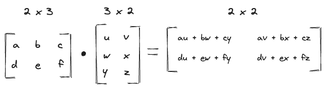
We will be going over a concrete example of this very soon.

Transpose

The transpose of a matrix involves flipping its rows into columns and its columns into rows. It is denoted as $A^{\text{T}}$.

If a matrix $A$ has dimensions $m \times n$ (i.e., $m$ rows and $n$ columns), its transpose $A^{\text{T}}$ will have dimensions $n \times m$ (i.e., $n$ rows and $m$ columns).

For a $2 \times 3$ matrix $A$:

$$A = \begin{bmatrix} 1 & 2 & 3 \\ 4 & 5 & 6 \end{bmatrix}$$

The transpose $A^{\text{T}}$ is a $3 \times 2$ matrix:

$$A^{\text{T}} = \begin{bmatrix} 1 & 4 \\ 2 & 5 \\ 3 & 6 \end{bmatrix}$$

Flipping images

This is actually how we flip images.

If we were to convert an image into a matrix as such:

def image_to_matrix(image_path: str):
    from PIL import Image

    image = Image.open(image_path)
    image = image.convert('L')

    image = np.array(image)
    return image

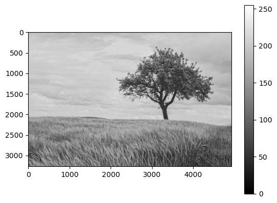
and then load and show the image:

image = image_to_matrix('tree.jpg')

show_matrix(image)

We get the following:

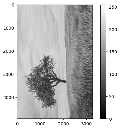
if we were to instead show the transpose:

show_matrix(image.T)

We see the image flipped.

Symmetric images

Matrices that don't change after transposition are called symmetric matrices.

To make a matrix symmetric, we average the Matrix and its transpose: $A_{\text{symmetric}} = \frac{A + A^T}{2}$

Let's try to make our image symmetric. Since it's not square yet, we need to first crop it a bit:

square_image = image[0:3000, 0:3000]
show_matrix(square_image)

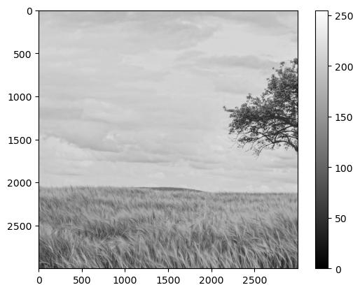
This is because we can't add 2 matrices with different dimensions.

Now if we Add the Matrix with it's transpose and divide by 2 we get:

symmetric_image = (square_image + square_image.T) / 2
show_matrix(symmetric_image)

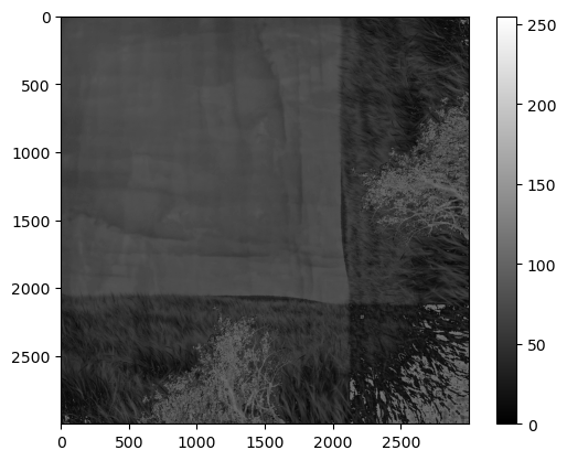
It looks weird, but it's correct. Id we were to show it's transpose, it's the same.

Perceptron (Neural Network) example

Before we continue, we actually have enough information already to calculate ourselves the most simplest kind of Artificial Neural networks: The perceptron. So I really want to emphasize the real world value you get with this by showing you exactly this calculation already.

A perceptron is the simplest type of neural network. It is a binary classifier that determines whether an input belongs to one class or another.

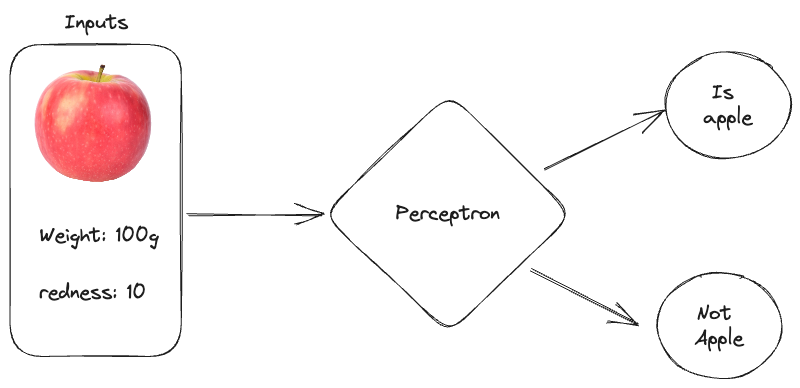
The perceptron works by calculating a weighted sum of the inputs, adding a bias, and passing the result through an activation function (like a step function).

Let's classify whether a fruit is an apple or not based on two features:

1. Weight (grams)

2. Redness (scale from 0 to 10, where 10 is fully red)

3. Inputs ( x ): • $x_1$: Weight of the fruit. • $x_2$ : Redness of the fruit.

4. Weights ( w ): • $w_1$: How important the weight is for classification. • $w_2$: How important the redness is for classification.

5. Bias ( b ): • A constant to shift the decision boundary.

6. Output ( y ): • $y = 1$ : The fruit is classified as an apple. • $y = 0$ : The fruit is not an apple.

The perceptron calculates a value z as:

$z = w_1 x_1 + w_2 x_2 + b$

Then applies an activation function to decide the output:

$$y = \begin{cases} 1 & \text{if } z \geq 0 \\ 0 & \text{if } z < 0 \end{cases}$$

Example

Input features: Weight of the fruit = 150 grams. Redness of the fruit = 8.

Input vector:

$$\mathbf{x} = \begin{bmatrix} 150 \\ 8 \end{bmatrix}$$

Now let us define some initial Weights. These basically show the algorithm how important each variable is for guessing the fruit. Weights are one thing that the training algorithm tries to find out by itself. For now let's define them freely as such:

$$\mathbf{w} = \begin{bmatrix} 0.02 \\ 0.5 \end{bmatrix}$$

Similarly, biases are also calculated by the training algorithm. Again, we'll define them freely as such: $b = -5$

So to calculate whether the fruit with 150g and 8 redness is a apple, we do the following:

$z = \mathbf{w}^{\text{T}} \cdot \mathbf{x} + b$ $z = \begin{bmatrix} 0.02 & 0.5 \end{bmatrix} \cdot \begin{bmatrix} 150 \\ 8 \end{bmatrix} + (-5)$ $z = (0.02 \cdot 150) + (0.5 \cdot 8) + (-5)$ $z = 3 + 4 - 5$ $z = 2$

Apply the step function:

$$y = \sigma(z) = \begin{cases} 1 & \text{if } z \geq 0 \\ 0 & \text{if } z < 0 \end{cases}$$

Since $z = 2 \geq 0$, $y = 1$

Meaning, it's probably an apple!

Determinant

Cofactor

Inverse Matrices

Even if we know that a matrix is invertible, it is usually difficult to compute its inverse.

The inverse of $A$, if it exists, is a matrix such that $AA^{-1} = A^{-1}A = I_n$. If an inverse exists, then we call a matrix invertible.

This inverse will be the ultimate tool to solve certain systems of linear equations.

Systems of Linear Equations

Instead of just teaching you why this section is important, let me show you it directly. Let's revisit the perceptron example with apples and explicitly connect it to solving systems of linear equations.

Suppose we have the following training data for classifying apples:

Feature 1: Weight (g)	Feature 2: Redness (on a scale of 1-10)	Output (1 = apple, 0 = not apple)
150	8	1
120	6	1
200	3	0
100	7	0

If you remember, the formula for perceptrons looks like this:

$y = \sigma(z) = \sigma(\mathbf{w}^{\text{T}} \cdot \mathbf{x} + b)$

Where $\sigma$ is the step function, $\mathbf{w}^{\text{T}}$ is the Weights matrix, $\mathbf{x}$ is the Input and $b$ is the bias.

The step function works like this: For $y = 1$, we want: $z_i \geq 0$ For $y = 0$, we want: $z_i < 0$

Now we want to find our weights and biases to finalize our Algorithm of classifying Apples in fruits.

From the data:

1. $150w_1 + 8w_2 + b \geq 0$
2. $120w_1 + 6w_2 + b \geq 0$
3. $200w_1 + 3w_2 + b < 0$
4. $100w_1 + 7w_2 + b < 0$

But how can we now finally get these? This is what we will explore in this section.

Introduction to Systems of Linear equations

The premise of this is finding unknown variables in equations.

If we were to take our 4 equations from our example.

1. $150w_1 + 8w_2 + b \geq 0$
2. $120w_1 + 6w_2 + b \geq 0$
3. $200w_1 + 3w_2 + b < 0$
4. $100w_1 + 7w_2 + b < 0$

We call $w_1$, $w_2$, and $b$ variables and the data (e..g. 150, 8, 0) coefficients of the system.

Out of this, we can actually create a Coefficient and a variable matrix as such:

$$A = \begin{bmatrix} 150 & 8 & 1 \\ 120 & 6 & 1 \\ 200 & 3 & 1 \\ 100 & 7 & 1 \end{bmatrix}, \quad \mathbf{w} = \begin{bmatrix} w_1 \\ w_2 \\ b \end{bmatrix}, \quad \mathbf{y} = \begin{bmatrix} 1 \\ 1 \\ 0 \\ 0 \end{bmatrix}$$

To get the weights and biases, we aim to solve:

$A \cdot \mathbf{w} = \mathbf{y}$

Meaning:

$$\begin{bmatrix} 150 & 8 & 1 \\ 120 & 6 & 1 \\ 200 & 3 & 1 \\ 100 & 7 & 1 \end{bmatrix} \cdot \begin{bmatrix} w_1 \\ w_2 \\ b \end{bmatrix} = \begin{bmatrix} 1 \\ 1 \\ 0 \\ 0 \end{bmatrix}$$

Such systems may have no solution, a unique solution or infinitely many solutions.

Before we solve our apple classifier, let's first go through some underlying theory of solving these equations first.

Gaussian elimination

Gaussian Elimination is a way to solve linear equations by manipulating matrices.

There are 3 ways allowed to manipulate the matrices:

1. Changing the order of the equation
2. Multiplying an equation with a scaler
3. Adding a multiple of an equation to another

By doing this, we hope to bring the equations matrix to a much simpler form to easily solve them.

The form we're trying to bring the matrix to is called a row echelon form. In there, three things need to be specified:

1. Zeros below the pivots: Each row starts with a leading non-zero number (called a pivot), and all rows below that row have zeros in that column.
2. Staircase pattern: The pivot in each row is to the right of the pivot in the row above, forming a staircase-like pattern.
3. All-zero rows (if any) are at the bottom: If there are rows where all elements are zero, they must be at the bottom of the matrix.

Given a $3 \times 3$ matrix:

$$\text{Original Matrix: } \begin{bmatrix} 2 & 4 & -2 \\ 4 & 9 & -3 \\ -2 & -3 & 7 \end{bmatrix}$$

After performing Gaussian elimination (row operations), we get:

$$\text{Row Echelon Form: } \begin{bmatrix} 1 & 2 & -1 \\ 0 & 1 & -0.5 \\ 0 & 0 & 1 \end{bmatrix}$$

There is also a reduced row echelon form, which looks like such:

$$\begin{bmatrix} 1 & 0 & 0 \\ 0 & 1 & 0 \\ 0 & 0 & 1 \end{bmatrix}$$

Having the Coefficient matrix in Row echelon form is really just like saying x = ?. y = ?, z = ?, meaning we solved it. That's kinda the goal of Gaussian elimination.

Imagine you are have 3 Equations and 3 unknown variables as such:

$$7x + 5y + 9z = -1$$ $$4x - 8y + 4z = -9$$ $$9x - 5y + 5z = -2$$

Transforming it using the 3 rules as mentioned before into Reduced Row Echelon Form gives you:

This is the same as saying:

$$x = 1.142..., y = 0.936..., z = -1.519...$$

Meaning we solved the system!

You can think of this as a Puzzle game, like Sudoku. Where the End state is a Matrix should be in row echelon form to be able to find the unknown variables.

This way of thinking brings a playful approach to these problems, as they are common questions in Linear Algebra tests.

Let's however now solve our Problem to get the weights and biases:

$$\begin{bmatrix} 150 & 8 & 1 & 1 \\ 120 & 6 & 1 & 1 \\ 200 & 3 & 1 & 0 \end{bmatrix}$$

We actually just need 3 samples of the data for this.

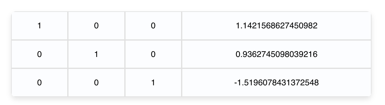
If we were to use Gaussian elimination, we would get the following Results:

$$w_1 = -0.01, w_2 =0.12, b =1.24$$

Putting this back into our Perceptron neural network, we get:

$z = (-0.01 \cdot x_1) + (0.12 \cdot x_2) + 1.24$

As our Classifier. With the data given.

Let's try this out with test sample. A strawberry has about 13.6g and a "redness" value of 10.

$z = (-0.01 \cdot 13.6) + (0.12 \cdot 10) + 1.24 = 2.304$

Ok not the best... It seems like it thinks that a strawberry is an apple.

This is because we only used 3 samples. The partial system we solved told the perceptron that redness is extremely important. This is when we would need to add more data to get better weights and biases. However this wouldn't be possible with Gaussian elimination.

Gaussian elimination typically works for square systems of linear equations (where the number of variables equals the number of equations). However, in our case, you have 4 samples (equations) but only 3 variables ( $w_1$, $w_2$, $b$ ), making it an overdetermined system.

The scope of which is outside of this video

Rank of a Matrix

The number of independent rows or independent columns in the matrix. It tells us how much "information" the matrix contains. It's basically the count of actual useful rows in a Linear System of equations.

Think of rank as the number of dimensions the matrix spans. For example:

• A rank of 2 means the matrix describes a 2D plane.
• A rank of 3 means it describes a 3D space.

The rank of determines:

1. If the system has no solutions, a unique solution, or infinitely many solutions.
2. Whether all the rows (or equations) are useful for solving, or if some rows are redundant (dependent).

• Full Rank: If the matrix A has full rank ($\text{rank}(A) = n$), it spans the entire space. This means we can solve $Ax = b$ uniquely for any $b$.
• Not Full Rank: If $\text{rank}(A) < n$, it doesn't span the full space. Some equations are redundant, leading to no solutions or infinitely many solutions.

$$A = \begin{bmatrix} 1 & 2 \\ 2 & 4 \end{bmatrix}, \quad \text{rank}(A) = 1$$

The second row is a multiple of the first ($2 \times \text{row}_1 = \text{row}_2$).

The system $Ax = b$ might have no solution (if $b$ is inconsistent with the equations) and it might have infinitely many solutions (if $b$ lies on the span of the rows).

Elementary matrices

An elementary matrix is just the Identity Matrix ($I_n$) with one row operation applied to it. Any row operation you perform on a matrix is the same as multiplying that matrix by an elementary matrix on the left. This means row operations are just matrix multiplications with a special kind of matrix!

a) Row Interchange Suppose we swap $R_1$ and $R_2$. The corresponding elementary matrix is:

$$E = \begin{bmatrix} 0 & 1 & 0 \\ 1 & 0 & 0 \\ 0 & 0 & 1 \end{bmatrix}$$

b) Row Scaling Suppose we scale $R_2$ by multiplying it by 3. The elementary matrix is:

$$E = \begin{bmatrix} 1 & 0 & 0 \\ 0 & 3 & 0 \\ 0 & 0 & 1 \end{bmatrix}$$

c) Row Replacement Suppose we replace $R_3$ with $R_3 + 4R_1$. The elementary matrix is:

$$E = \begin{bmatrix} 1 & 0 & 0 \\ 0 & 1 & 0 \\ 4 & 0 & 1 \end{bmatrix}$$

Inverse matrices

The last topic we will cover is getting the inverse of a matrix. One of the main motivations for working with the inverse matrix is that it can be used to solve linear systems in a straightforward way. Super important for this simple trick right here:

If $A \cdot \mathbf{x} = \mathbf{b}$, you multiply by the inverse to get: $\mathbf{x} = A^{-1} \cdot \mathbf{b}$

Meaning, we can get the unknowns without doing gaussian elimination, and instead just simply doing a dot product. That's great! As this would help us get our weights and biases for our Neural Network.

Solving Inverses

There are 2 main ways of calculating the inverse of a matrix:

1. Gaussian Elimination
2. Cofactor expansion

You can pick which one works for you best.

Gaussian elimination to find inverses

This method builds the inverse step by step by transforming A into the identity matrix I. Along the way, we construct $A^{-1}$.

Steps:

1. Set up an augmented matrix: $[A | I]$, where I is the identity matrix.
2. Apply row operations to reduce A to I, while applying the same operations to I.
3. Result: Once A becomes I, the transformed I becomes $A^{-1}$.

Example:

$$A = \begin{bmatrix} 1 & 2 \\ 3 & 4 \end{bmatrix}$$

Step 1: Augment with I:

$$\left[ \begin{array}{cc|cc} 1 & 2 & 1 & 0 \\ 3 & 4 & 0 & 1 \end{array} \right]$$

Step 2: Row reduce A to I:

$$R_2 = R_2 - 3R_1 \quad \Rightarrow \quad \left[ \begin{array}{cc|cc} 1 & 2 & 1 & 0 \\ 0 & -2 & -3 & 1 \end{array} \right]$$ $$R_2 = -\frac{1}{2}R_2 \quad \Rightarrow \quad \left[ \begin{array}{cc|cc} 1 & 2 & 1 & 0 \\ 0 & 1 & \frac{3}{2} & -\frac{1}{2} \end{array} \right]$$ $$R_1 = R_1 - 2R_2 \quad \Rightarrow \quad \left[ \begin{array}{cc|cc} 1 & 0 & -2 & 1 \\ 0 & 1 & \frac{3}{2} & -\frac{1}{2} \end{array} \right].$$

Step 3: Result:

$$A^{-1} = \begin{bmatrix} -2 & 1 \\ \frac{3}{2} & -\frac{1}{2} \end{bmatrix}$$

Cofactor Expansion for finding inverses

The general formula for this is the following:

$$A^{-1} = \frac{1}{\text{det}(A)} \cdot C^T$$

Now there is a lot to unpack here since there are a lot of new things. What is det(A) supposed to mean? What is this weird $C^T$? We'll cover all that now. You will get to see however, that this option might be the easier one actually. The reason being is that its actually just a Scalar multiplication in the end.

But let's not get ahead of ourselves. Let's go through each part of this equation to understand what it means.

The Determinant

The determinant of a square matrix (A) is a single number that provides key information about the matrix, such as:

1. Scaling: How the matrix transforms space (e.g., stretches, flips, or collapses it).
2. Invertibility: Whether the matrix can be inverted (useful in solving systems of equations).

For now, just see this as a necessary matrix operation needed for getting the inverse.

Calculating the determinant is a bit tricky and not that intuitive. We begin with 2x2 Matrices as they are the easiest to calculate for the determinant.

$$A = \begin{bmatrix} 3 & 2 \\ 1 & 4 \end{bmatrix}, \text{det}(A) = (3)(4) - (2)(1) = 12 - 2 = 10$$

For larger matrices we have to do something called cofactor expansion.

$$A = \begin{bmatrix} a_{11} & a_{12} & a_{13} \\ a_{21} & a_{22} & a_{23} \\ a_{31} & a_{32} & a_{33} \end{bmatrix}$$

I personally remember the following process to properly calculate the determinant of larger matrices:

1. Pick a row, preferably with many zeros.
2. Go through each element of the row and remove the row and column to it

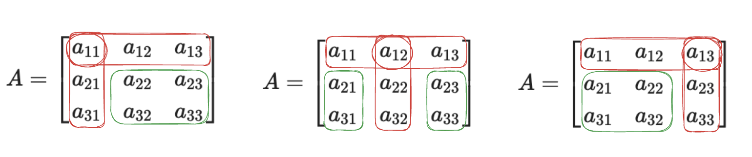
3. Calculate the determinant of the resulting smaller matrix.

$$\text{det}(A) = a_{11} \cdot \text{det}(A_{11}) - a_{12} \cdot \text{det}(A_{12}) + a_{13} \cdot \text{det}(A_{13})$$

One important thing to note here is the sign. While there is a formula for getting the sign, the intuitive way is to simply remember this: Row number + Column number (e.g. row 1 column 2). If this is odd, then the sign is negative, else it is positive. Or even simpler:

This will be also important for getting the Cofactor, the next step of the Matrix inverse equation.

Example:

$$A = \begin{bmatrix} 1 & 0 & 2 \\ 4 & 1 & 8 \\ 0 & 1 & 1 \end{bmatrix}$$ $$\text{det}(A) = 1 \cdot \text{det}\begin{bmatrix} 1 & 8 \\ 1 & 1 \end{bmatrix} - 0 \cdot (\dots) + 2 \cdot \text{det}\begin{bmatrix} 4 & 1 \\ 0 & 1 \end{bmatrix}$$ $$\text{det}(A) = 1 \cdot (1 - 8) + 2 \cdot (4 - 0) = -7 + 8 = 1$$

Cofactor of a Matrix

A cofactor of an element in a matrix is a value that combines:

1. The minor of the element (the determinant of the smaller matrix obtained by removing the element’s row and column).
2. A sign adjustment based on the element’s position.

It's kinda easier to show than to explain. Let's take the same matrix from the previous example:

$$A = \begin{bmatrix} 1 & 0 & 2 \\ 4 & 1 & 8 \\ 0 & 1 & 1 \end{bmatrix}$$

To get the Cofactor matrix, we need to calculate the determinant of every single element in the matrix and then substituting the element with it's determinant counterpart. This sentence isn't quite accurate but it helps me think about it.

This is the general intuitive algorithm:

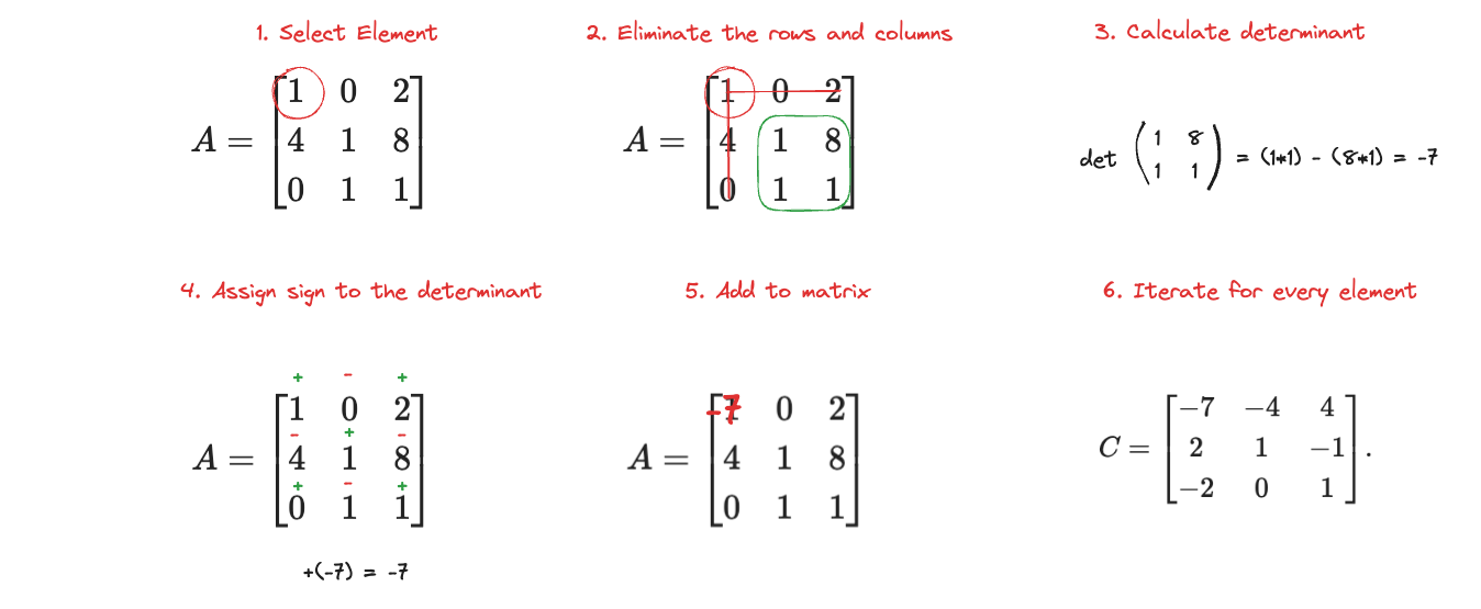
After doing so with every element, we get the cofactor matrix as such:

$$C = \begin{bmatrix} -7 & -4 & 4 \\ 2 & 1 & -1 \\ -2 & 0 & 1 \end{bmatrix}$$

To now finally get the inverse of a matrix, we multiply the transpose of this matrix by the scalar of $\frac{1}{\text{det}(A)}$

So the Transpose $C^T$ (flipped matrix) is:

$$C^T = \begin{bmatrix} -7 & 2 & -2 \\ -4 & 1 & 0 \\ 4 & -1 & 1 \end{bmatrix}$$ $$A^{-1} = \frac{1}{\text{det}(A)} \cdot C^T = C^T = \frac{1}{1} \begin{bmatrix} -7 & 2 & -2 \\ -4 & 1 & 0 \\ 4 & -1 & 1 \end{bmatrix} = \begin{bmatrix} -7 & 2 & -2 \\ -4 & 1 & 0 \\ 4 & -1 & 1 \end{bmatrix}$$

And that's it! We've successfully found the inverse through cofactor expansion!