Collaborative Filtering

As we discused earlier, this type is more like a democracy. Here, the algorithm uses user interactions, like likes or views of an item, to determine whether it should recommend the item or not.

You can think of this like the algorithm that pushes to you content on TikTok or YouTube of currently trending videos which might interest you.

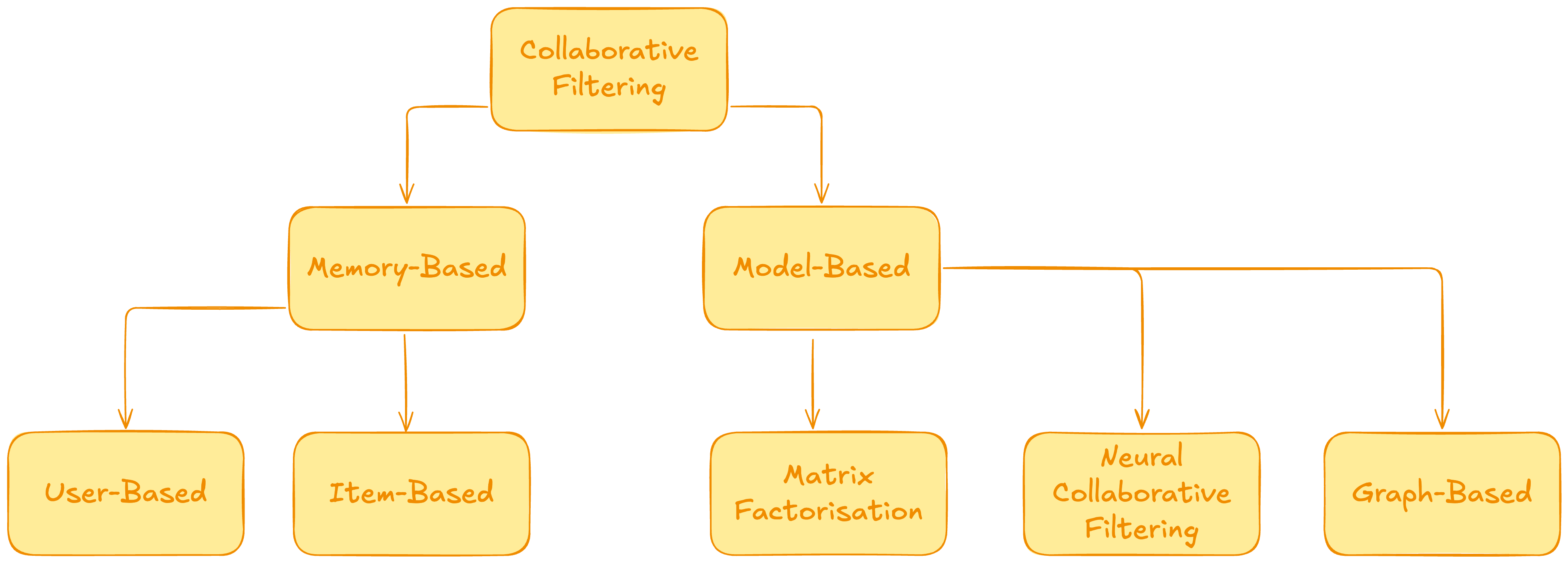
In this lesson, we will go over the following:

1. Memory-Based approaches
2. Model-Based approaches
3. Graph-Based approaches

Memory-Based Collaborative filtering

Imagine you have a small dataset of users, and items which they ranked from 1-5:

User	Item A	Item B	Item C
Alice	5	3	—
Bob	4	2	5
Carol	1	5	4

"Alice" hasn't rated Item C, our job is to predict how much she would like it.

This is what we would call User-Based, in contrast to Item-Based where we would try to find users instead, which would like an item.

However both approaches are relatively the same. For this we generally follow 2 steps: First we calculate the similarities between other users, and then we compute the weighted average.

Here is how this would look like:

1. Finding similar Users

To do this, we simply create vectors out of the users based on their ratings and then use cosine similarity, like in the content-based approaches:

$$Alics = (5, 3), Bob = (4, 1), Carol=(1, 5)$$

If we were to then find the similarity between the users, we would get:

$$sim(Alice, Bob) = 0.997; sim(Alice, Carol) = 0.673$$

As we can see, Alice is a lot closer to Bob than Carol from her past Item ratings.

We then take these similarities and the ratings of past users to see how much Alice would like it. In our example, Bob rated Item C with 5, since Alice is very close with bob, we multiply his rating with $0.997$. Similarly, we take Carols rating of 4 for Item C and multiply it by $0.673$, which was her similarity rating.

We then take the average, as such:

$$\frac{0.997 * 5 + 0.673 * 4}{0.997 + 0.673} = 4.59$$

Which means, our estimate for Alices rating for Item C is $4.59$.

Like mentioned earlier, Item-based would basically be the same, but the other way around. Instead of seeing how much Alice would like Item C, we would try to find similar Items, not users. So the vector would include an Items ratings of all users, instead of a users rating of all Items.

Model-Based Collaborative filtering

While Memory-Based approaches only really used some small vector math, model based are a bit more sophisticated. It's all about training a model on the user–item interaction data to learn the hidden factors that explain why users like certain items, and then use that model to predict new preferences.

These are the models which really feel scary, like they know exactly what you want.

Matrix Factorisation

This method is one of the most widely used ones. Imagine we have the following data:

	Item A	Item B	Item C
Alice	5	3	–
Bob	4	–	5
Carol	1	5	4

What we do now is basically create hidden, imaginary features. The amount of which is just a hyperparameter, so we can just play around with how many made up features we want. These imaginary features we call "Latent Factors". We initialize them with random values for both the items and features:

	Feature 1	Feature 2
Item A	1.2	3
Item B	4.1	2
Item C	3.1	5.1
Alice	5.1	3
Bob	4	2.1
Carol	1	5

We then calculate with these random numbers the similarity between Item and User. To do this we can again use Cosine similarity.

So for instance, The similarity between Alice (5.1, 3) and Item A (1.2, 3) is 0.79, and for Carol and Item A, it is 0.98.

We calculate all the User-Item similarities and then compare on how they did compared to what was actually liked. e.g. if $sim(Alice, Item A)$ is close to one ($0.79$), it means the user will like it a lot. Which we do see, as Alice rated Item A with a 5. However since we randomized the values, it cant all be right on the first try. As we can see, Carol didnt like Item A, however got a similarity for it of $0.98$, meaning our model would falsely recommend it to her.

To combat this we calculate an error for each, and then update these values based on the error. This will get our latent factors closer to what it actually is.

Neural Collaborative Filtering

This builds on top of matrix factorization. It uses a neural network to learn the hidden features of the users and dishes.

So instead of just using a similarity calculation, it feeds it into its own tiny neural network to produce the prediction. To do this, it uses as an input the user and the item features, then feeds it through a Multi Layer Perceptron, and then it just uses the sigmoid function to get an output between 0 and 1.

We then train this network and thats it.

Graph-Based methods

These are great for capturing complex relationships between users and items.

Instead of looking at users and items separately, Graph models treat the entire system as a network of users and items connected by interactions.

• Every user and every item is a node.
• Every purchase is a connection (edge) between them.

Then, we spread signals across this graph to recommend new items.

In general, there are 2 ways of getting recommendations from Graph-based models. One of them is to create a bipartate graph based on the user-item interactions, and then using a Graph model to fetch predictions.

The other way would be to make a full social network, to then try to see what similar users around you like, to then recommend that to you.

Imagine you have this graph:

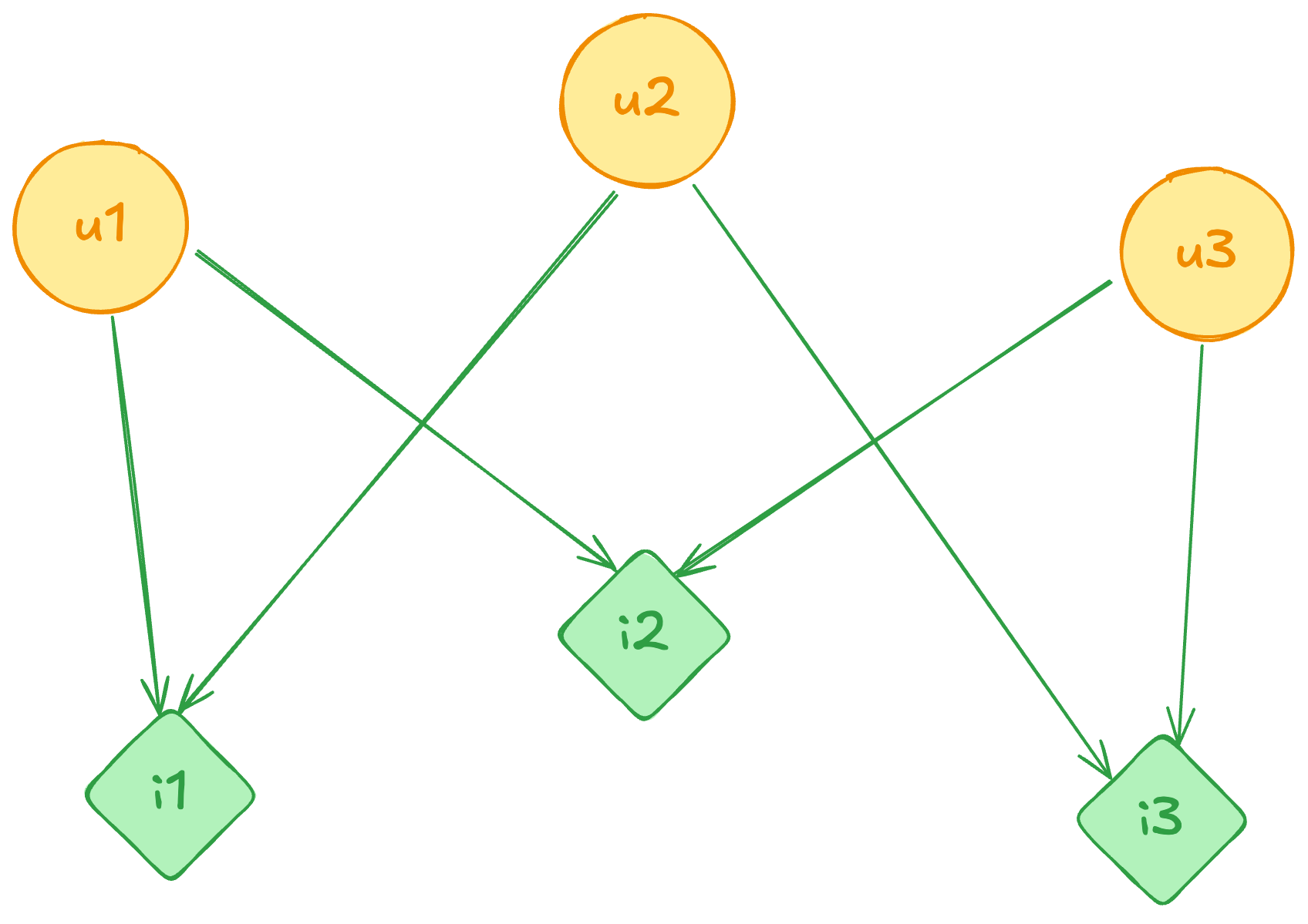
Models, like the two-hop Neighbor algorithm, would look for the closest users to them, and then their closest neighbors, to predict the next most probable item. E.g. if you and your friends all like Shawarma, and 3 of your friends have also liked Milkshakes, then you would get Milkshakes as a recommendation.

In the approach of using graph neural networks instead, we want to learn embeddings for each node so that we can score unseen edges (e.g., recommend I3 to U1).

To do this we first initialize node features with random numbers:

Node	Initial feature
U1	1.0
U2	2.0
U3	3.0
I1	4.0
I2	5.0
I3	6.0

In practice these could be multi-dimensional, coming from user profiles or item metadata.

Each node collects ("receives") its neighbors' features and averages them to form a new feature:

Node	New feature (Layer 1)
U1	(4.0+5.0)/2 = 4.5
U2	(4.0+6.0)/2 = 5.0
U3	(5.0+6.0)/2 = 5.5
I1	(1.0+2.0)/2 = 1.5
I2	(1.0+3.0)/2 = 2.0
I3	(2.0+3.0)/2 = 2.5

We repeat the process, but now using Layer 1 features. E.g:

U1's neighbors now have features $I1'=1.5, I2'=2.0.$ Therefore:

$U1" = (1.5 + 2.0) / 2 = 1.75$

I3's neighbors are $U2'=5.0 and U3'=5.5.$ Therefore: $I3" = (5.0 + 5.5) / 2 = 5.25$

After two layers, each node has "looked" out two hops and blended features from farther away.

Now we have final embeddings for users and items. To recommend. We then similarly just compute the similarities of these vectors.

Item	Final feature (Layer 2)	Similarity to U1" (1.75)
I1	…	…
I2	…	…
I3	5.25	high

Since I3"=5.25 is much closer to U1"=1.75 than I1" or I2" would be, I3 becomes the top recommendation for U1.