Factor Analysis

Imagine you run a Shawarma resteraunt and you’ve collected these scores (from 100 customers) on six different variables:

Observable Rating	Description
Juiciness	How succulent the meat is
Spice Level	How well the spices hit the tongue
Wrap Tightness	How neatly the wrap holds together
Staff Friendliness	How warm the service feels
Wait Time	Minutes until you get your wrap
Price Fairness	Perceived value for money

These six ratings often move together. But you suspect there are just two big variables driving all that:

• Food Quality (meat + spices + wrap)
• Service Experience (friendliness + speed + value)

These guesses are called latent factors.

Factor Analysis teases out exactly those unobserved latent factors (Food Quality & Service Experience) that explain why those six numbers are correlated, so you can simplify your menu feedback into two clear metrics.

Basically saying, Factor Analysis is a technique that allows us to reduce the number of variables in a dataset by identifying underlying patterns and relationships.

Motivation

FA assumes each observed rating (e.g., Juiciness) is made of a shared part driven by a few hidden factors (like “Food Quality”), and a unique part (noise) that’s just measurement error, typos, or quirky tastes. Why does it matter? Suppose one customer fat-fingered their Spice Level rating. FA automatically treats that as “unique noise” and keeps it from skewing your overall Food Quality factor.

Also, in real surveys, some questions are “noisier”, e.g. customers vary wildly on Price Fairness but are consistent on Juiciness. FA models those different noise levels explicitly. Why does that matter? If Price Fairness is super noisy, FA down-weights its influence on your latent “Service Experience” factor. That keeps your factor scores more stable.

But I think the coolest thing about FA is that it allows us to actually just speak in normal language about the actionable insights we can take from the data. So FA can tell you that "Juiciness loads 0.8 on Food Quality" and "Wait Time loads 0.9 on Service Experience". That is super practical and useful.

How FA Differs from PCA

One of the main problems with PCA is that it doesn't take into account the noise in the data. Factor Analysis on the other hand, explicitly models unique variance (noise) separately from common variance (signal), giving you cleaner, more trustworthy factors. Also it very nicely is able to map to theoretical constructs (e.g. “Quality”).

I remember when I first learned about PCA, it was very difficult for me to grasp what exactly these new variables were. It took me a while to understand that they were just a mathematical construct to help us understand the data better. This would have been much easier to understand if I had known about Factor Analysis beforehand.

The Data

We will be using a 6x100 test Dataset which has been generated by ChatGPT.

Here is how it looks like:

Juiciness	Spice Level	Wrap Tightness	Staff Friendliness	Wait Time (min)	Price Fairness
6.5	7.2	8.1	8.9	10.2	7.4
5.8	6.1	7.5	7.8	12.3	6.8
…	…	…	…	…	…
7.3	8.4	8.7	9.1	9.5	8.0

Download the full dataset here

1. Data Preparation

Before we can perform Factor Analysis, we need to prepare the data. What we need to do is to scale the data so that each variable has a mean of 0 and 1. Meaning, if we take our data, and we have the minimum spiciness score as 1 and the maximum spiciness score as 10, we need to scale it so that the minimum spiciness score is 0 and the maximum spiciness score is 1.

We can do this by using the MinMaxScaler from sklearn.preprocessing.

scaler = MinMaxScaler()
scaled_data = scaler.fit_transform(data)

What we then could do is create a correlation matrix to see how the variables are correlated with each other. This is done mathematically by taking the dot product of the scaled data with itself.

$$\mathbf{R} = \mathbf{X}^T \mathbf{X}$$

In code, this looks like this:

correlation_matrix = scaled_data.T @ scaled_data

This is what we get:

	Juiciness	Spice Level	Wrap Tightness	Staff Friendliness	Wait Time (min)	Price Fairness
Juiciness	1.000	0.695	0.869	–0.199	0.102	–0.161
Spice Level	0.695	1.000	0.734	–0.156	0.143	–0.188
Wrap Tightness	0.869	0.734	1.000	–0.135	0.106	–0.117
Staff Friendliness	–0.199	–0.156	–0.135	1.000	–0.701	0.807
Wait Time (min)	0.102	0.143	0.106	–0.701	1.000	–0.675
Price Fairness	–0.161	–0.188	–0.117	0.807	–0.675	1.000

We then can see which variables are correlated with each other. For example, Juiciness, Spice, Wrap are strongly positively correlated and Friendliness, Wait Time, Price Fairness form a correlated block.

Next we will determine the number of factors to extract.

2. Determine the Number of Factors

To determine the number of factors to extract, we can use the scree plot. This is a plot of the eigenvalues of the correlation matrix.

But what are eigenvalues and why do we need them?

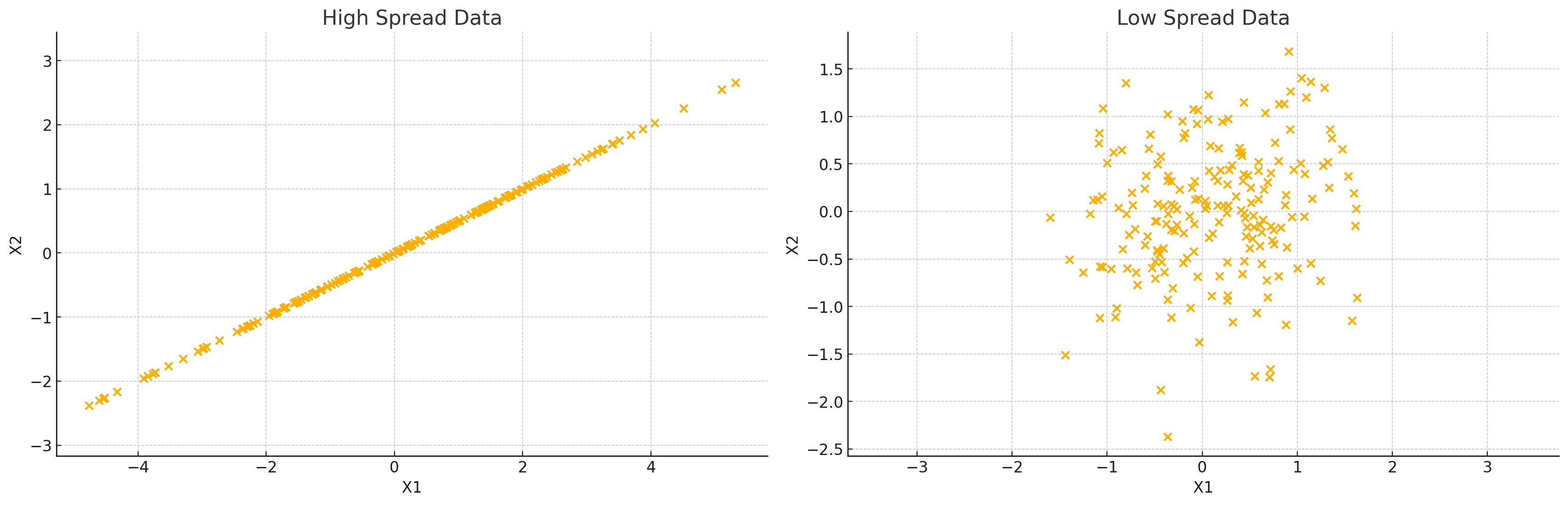
Eigenvalues are a measure of the importance of each factor. The higher the eigenvalue, the more important the factor. An eigenvalue measures "how much spread" in our data a single factor would explain if it were aligned with that eigenvector direction. Which basically means that the higher the eigenvalue, the more spread in our data that factor explains.

To get the eigenvalues, we use the following fomula on our correlation matrix:

$$\mathbf{R} \mathbf{v} = \lambda \mathbf{v}$$

Where:

• $\mathbf{R}$ is our correlation matrix
• $\mathbf{v}$ is our eigenvector
• $\lambda$ is our eigenvalue

In python, this looks like this:

eigenvalues, eigenvectors = np.linalg.eig(correlation_matrix)

The eigenvalues are then:

Feature	Eigenvalue
1	2.934
2	2.060
3	0.363
4	0.336
5	0.122
6	0.184

Kaiser Criterion

We only keep the factors with an eigenvalue greater than 1. This is because we want to keep only the factors that explain more than 100% of the variance in our data. This is called the Kaiser Criterion.

Scree Plot

We can also plot the scree plot to see the eigenvalues:

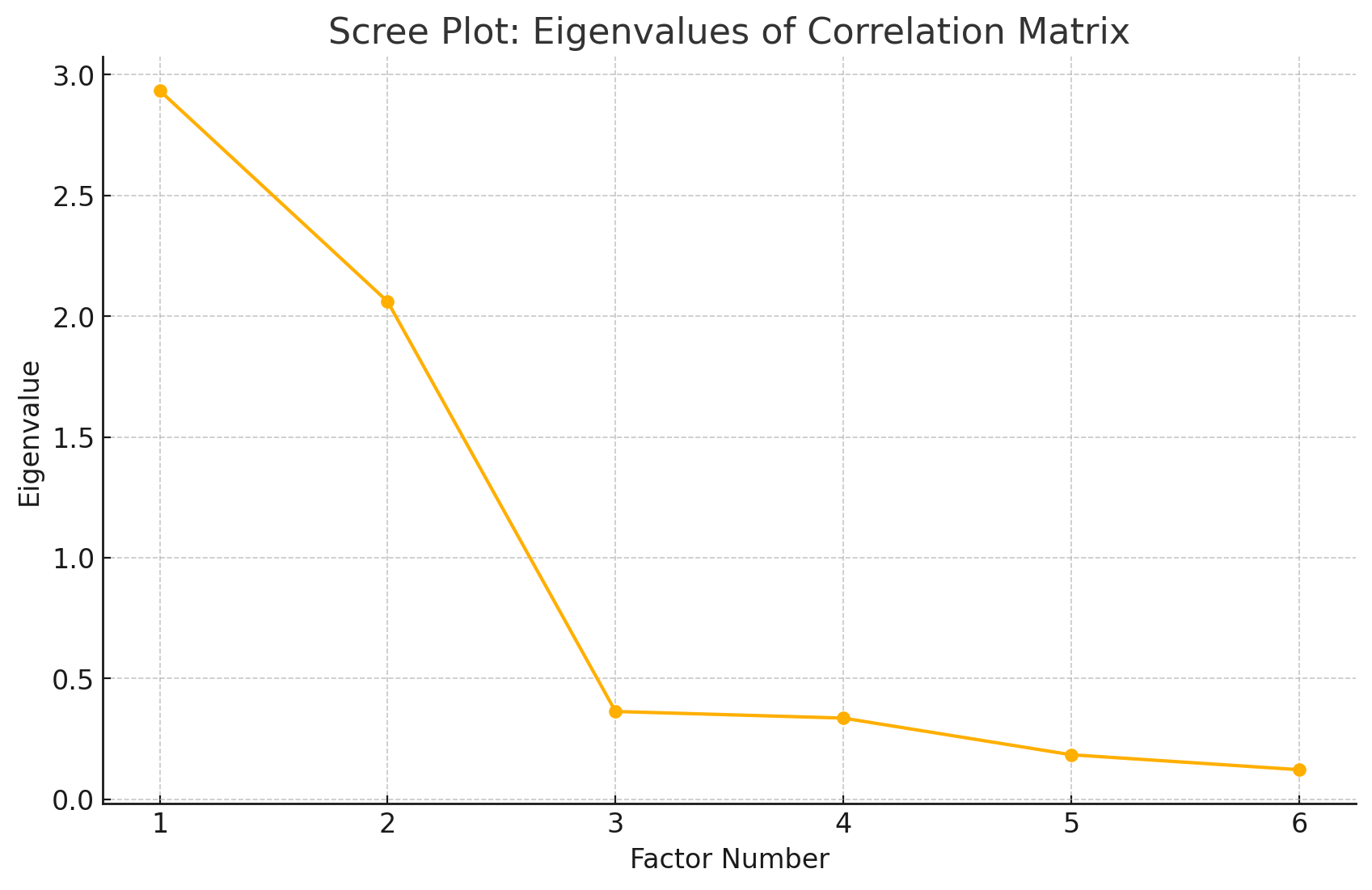
We can see that the eigenvalues are decreasing. This means that the factors are not explaining the data as well as the previous factor. We can see that the scree plot levels off at 2. This means that the first two factors are explaining the data as well as the previous factor.

Parallel Analysis

What if our big eigenvalues just happened by chance? We can use Parallel Analysis to determine the number of factors to extract.

Parallel Analysis is a technique that uses random data to determine the number of factors to extract.

1. We simulate (here, 100 times) completely random data with the same shape (100×6) and compute its eigenvalues.
2. We average those random eigenvalues—those are what “pure noise” would typically produce.
3. We only keep factors whose actual eigenvalue exceeds the noise average.

Factor	Actual EV	Noise Mean EV	Keep?
1	2.94	~1.35	Yes (2.94 > 1.35)
2	2.06	~1.17	Yes (2.06 > 1.17)
3	0.36	~1.05	No (0.36 < 1.05)
…	…	…	No

Putting it all together

So we now have a tripple check on the number of factors to extract:

Method	Factors Suggested
Scree-plot elbow	2 (steep drop after ➔ keep 1–2)
Kaiser (EV > 1)	2 (only 1 & 2 exceed 1)
Parallel analysis	2 (only 1 & 2 exceed random mean)

3. Factor Analysis model

Let's break down how we model the hidden factors that influence customer ratings of shawarma shops.

The Basic Model

For each shawarma shop visit, we collect 6 ratings:

• Juiciness
• Spice Level
• Wrap Tightness
• Staff Friendliness
• Wait Time
• Price Fairness

We believe these ratings are influenced by two hidden factors:

1. Food Quality - How well the shawarma is prepared
2. Service Experience - How good the overall service is

We can write this relationship as:

$$\mathbf{x} = \mathbf{B} \mathbf{f} + \mathbf{\epsilon}$$

Where:

• $\mathbf{x}$ is our 6 ratings (e.g., [7.2, 5.2, 5.8, 2.5, 16.0, 2.3])
• $\mathbf{B}$ is our loading matrix showing how each rating is influenced by food quality and service
• $\mathbf{f}$ is our two hidden factors [Food Quality, Service Experience]
• $\mathbf{\epsilon}$ is the error term (random variations in ratings)

Distribution of Hidden Factors

We assume the hidden factors follow a normal distribution centered at 0:

$$\mathbf{f} \sim \mathcal{N}(0, \mathbf{I})$$

This means:

• Most customers will give average ratings
• Some will give very high or very low ratings
• The distribution is symmetric around the mean

Example

For a customer who experienced:

• High Food Quality (f₁ = 1.5)
• Low Service Experience (f₂ = -0.8)

Their ratings would be influenced by these factors according to the loading matrix B, plus some random variation (ε).

This model helps us understand the underlying factors that drive customer satisfaction, even though we can't directly measure "Food Quality" or "Service Experience".

What we basically need to do is to find the best parameters for our factor analysis model. To do this, we will use the Expectation-Maximization (EM) algorithm.

Understanding the Likelihood and EM Algorithm

Let's break down how we find the best parameters for our factor analysis model in simpler terms:

The Complete Picture

Imagine you're trying to understand why someone gave certain ratings for their shawarma experience. There are two parts to this:

1. The ratings they gave (like juiciness, spice level, etc.)
2. The hidden reasons behind these ratings (like food quality and service experience)

If we could magically see both parts, we could write down how likely this combination is to happen. This is what we call the "joint probability" - it's like saying "what are the chances of seeing these specific ratings AND these specific hidden factors?"

We can break this down into two simpler questions:

• Given the hidden factors (like good food quality but bad service), how likely are these specific ratings?
• How likely are these hidden factors to occur in the first place?

It's like saying: "What are the chances of someone giving these ratings if they had this experience, AND what are the chances of them having this experience in the first place?"

Mathematically, this looks like this:

$$p(\mathbf{x}_n, \mathbf{f}_n) = p(\mathbf{x}_n | \mathbf{f}_n) \cdot p(\mathbf{f}_n)$$

This means:

• $p(\mathbf{x}_n | \mathbf{f}_n)$: How likely are these ratings given the hidden factors?
• $p(\mathbf{f}_n)$: How likely are these hidden factors?

The Problem

We can't directly observe the hidden factors! We only see the ratings. This makes finding the best parameters tricky.

The Solution: EM Algorithm

We use the Expectation-Maximization (EM) algorithm, which works in two steps:

1. E-step (Expectation)

   • Given our current guess of parameters
   • Calculate what we expect the hidden factors to be

2. M-step (Maximization)

   • Update our parameters to make the model fit better
   • Keep doing this until we can't improve anymore

This is like trying to find the best recipe for a dish:

• You can't directly measure the "perfect amount of spice"
• But you can keep adjusting and tasting until it's just right

The EM algorithm does something similar - it keeps adjusting the parameters until the model fits the data as well as possible.

Example

Let's use our shawarma ratings to see how EM works in practice:

1. Initial Guess

   • We start by guessing that there are 2 hidden factors:
     • Food Quality (affects juiciness, spice level, wrap tightness)
     • Service Experience (affects staff friendliness, wait time, price fairness)
   • We make an initial guess about how these factors relate to ratings

2. E-step (Expectation)

   • For each shawarma review, we estimate the hidden factors
   • Example: A review with high juiciness (9.4) and spice (9.0) but low staff friendliness (3.3)
     • We'd expect high Food Quality but low Service Experience

3. M-step (Maximization)

   • We update our model based on these estimates
   • If we see many reviews with high juiciness and spice but low staff friendliness
     • We adjust our model to better reflect this pattern

4. Repeat

   • We keep doing E and M steps until the model stops improving
   • Eventually, we get a clear picture of how Food Quality and Service Experience affect ratings

This is like a chef tasting a dish, adjusting the recipe, tasting again, and repeating until it's perfect!

Let's break this down with super simple numbers:

1. First Guess (Initial Parameters):

   • Food Quality Factor: 0.5 (middle value)
   • Service Factor: 0.5 (middle value)

2. E-Step (Looking at One Review):

   • Review Data:
     • Juiciness: 9/10
     • Spice: 9/10
     • Staff: 3/10
   • Our Guess:
     • Food Quality: 0.9 (high because food ratings are high)
     • Service: 0.3 (low because staff rating is low)

3. M-Step (Update Our Model):

   • Old Food Quality: 0.5 → New: 0.7
   • Old Service: 0.5 → New: 0.4 (We adjust these numbers based on what we learned)

4. Keep Repeating:

   • Do steps 2-3 for every review
   • Keep adjusting until numbers stop changing much
   • Final numbers might be:
     • Food Quality: 0.8
     • Service: 0.4

This then means that the best parameters for our factor analysis model are:

• Food Quality: 0.8
• Service: 0.4

And we can use this to predict the ratings for new reviews.

4. Implementing Factor Analysis in Python

Now that we understand the theory, let's implement it in Python.

We will be using sklearn to implement the factor analysis model.

from sklearn.decomposition import FactorAnalysis

fa = FactorAnalysis(n_components=2, random_state=42)
fa.fit(scaled_data)

# Get the loadings
loadings = fa.components_

print(loadings)

This will give us the loadings for each factor.

Factor 1: [-0.179, -0.152, -0.188, 0.073, -0.061, 0.074] Factor 2: [ 0.037, 0.027, 0.052, 0.159, -0.147, 0.168]

We interpret the loadings as follows:

• Factor 1:

  • Juiciness: -0.179
  • Spice: -0.152
  • Wrap Tightness: -0.188
  • Staff Friendliness: 0.073
  • Wait Time: -0.061
  • Price Fairness: 0.074

• Factor 2:

  • Juiciness: 0.037
  • Spice: 0.027
  • Wrap Tightness: 0.052
  • Staff Friendliness: 0.159
  • Wait Time: -0.147
  • Price Fairness: 0.168

This means that the first factor is influenced by Juiciness, Spice, Wrap Tightness and Price Fairness and the second factor is influenced by Staff Friendliness and Wait Time. Loadings close to 0 means that the factor is not influencing the rating.