Temporal Logic

Temporal logic is used by big companies, such as AWS, Azure and MongoDB to help find bugs in their systems.

What is Temporal Logic all about?

Temporal logic is simply a way to talk about how facts change over time, by extending regular "true/false" logic with a few special words—like "eventually" or "always"—to say when something should happen. Think of it as writing rules about a system's behavior along a timeline.

Classical logic can say "the light is on" or "the door is open", but not when those happen. Temporal logic adds operators that let you specify timing:

• X p ("next p"): in the next moment, p holds.
• F p ("finally p" or "eventually p"): at some point in the future, p will hold.
• G p ("globally p" or "always p"): from now on, p holds at every moment.
• p U q ("p until q"): p remains true until q becomes true.

Here some examples:

“A request is never left unanswered.”: G (request → F grant)

“Once the car’s engine is running, the brake must always work.”: G (engineOn → brakeOperational)

These precise rules can be automatically checked against a model of the system to catch design bugs before code is ever written.

The foundational idea was introduced by Amir Pnueli in 1977, formalizing how to reason about programs over time

Question 1 of 5

How can I show "eventually p" in temporal logic?

X pF pG pp U q

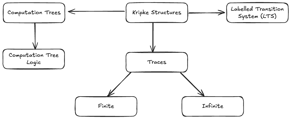
Kripke Structures

A Kripke structure is just a way to model all the possible states of a system and how you can move between them, plus which facts are true in each snapshot. You can then ask temporal logic questions like “Is it always true that … ?” or “Eventually, will … happen?”

There are 3 elements:

• States (nodes): describe a particular configuration (e.g. “traffic light is red”).
• Transitions (directed edges): describe how you can go from one state to another (e.g. “after red comes green”).
• Labels: each state carries a set of atomic propositions—simple true/false facts that hold in that state (e.g. in the “red” state, proposition isRed is true, isGreen is false).

Formal Definition

A Kripke structure K = (S, I, T, L) consists of:

• $S$: a finite set of states.
• $I ⊆ S$: a non-empty set of initial states where execution can start.
• $T ⊆ S × S$: a total transition relation—every state has at least one outgoing edge.
• $\mathscr{L} : S \rightarrow \mathcal{P}(\mathcal{A})$: a labeling function mapping each state to the set of atomic propositions $A$ true there.

Hardware, protocols, or concurrent software can all be modeled as Kripke structures.

Imagine this dummy example: Patt (P) and Quinn (Q) are two friends that share an apartment. They have one shared bathroom for the two of them.

There are 4 possible states:

• A: The bathroom is empty.
• B: Patt is in the bathroom.
• C: Quinn is in the bathroom.
• D: Both are in the bathroom. (Error state)

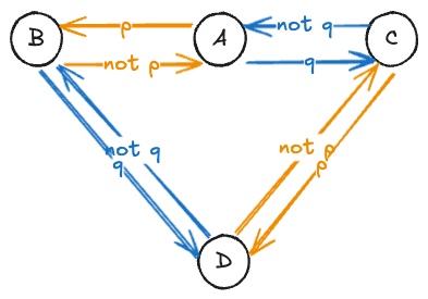
We want to be sure Pat and Quinn never end up in the bathroom at the same time. In this simple model:

Error State (D) is “Both In.” We can ask: “Is it always true that we never reach ‘Both In’?”

If our bathroom “model checker” finds a path like "Empty → Pat In → Both In", we know there’s a bug: no lock on the door.

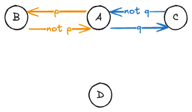
How can we fix this?: In our model, remove the transition “Pat In → Both In.” Now there’s no way to go from “Pat In” to “Both In.”

LTS (Labelled Transition System)

LTS are basically Kripke structures with a few extra features. They are used to model systems that can change states based on actions or events.

How You Turn an LTS into a Kripke Structure

States

In the new Kripke model, each state is a pair (oldState, lastAction).

This "bundles" the action into the state itself.

Initial States

If your LTS could start in state $s_0$ with no prior action, you introduce a dummy "start" action so your Kripke model's initial states are $(s_0,\text{"start"})$.

Transitions

Suppose in the LTS you have:

s ──a──► s′

Then in the Kripke structure you connect:

(s, a) ───► (s′, a′)

for every possible next action $a′$. Concretely, you allow any label in the "next" position so the transition relation is total.

Labels

In each new state $(s, a)$, you let the proposition $\text{lastWas}(a)$ be true. You can also carry over any facts about $s$ itself if you like.

Finite and Infinite traces

A trace is a sequence of states that a system can go through. It’s like a path through the Kripke structure.

Finite trace: stops after a few steps, e.g.

(wakeUp, brushTeeth, eatBreakfast, leaveHouse)

Infinite trace: goes on forever, e.g. your morning routine repeated every day

(wakeUp, brushTeeth, eatBreakfast, leaveHouse, wakeUp, brushTeeth, …) = (wakeUp, brushTeeth, eatBreakfast, leaveHouse)ᵠ

Finite traces model runs that end (e.g., a checkout process). Infinite traces model ongoing behavior (e.g., a web server that never stops).

LTL (linear‐time temporal logic) talks about properties of traces: G p (“always p”): p holds in every state of the trace. F p (“eventually p”): p holds in at least one later state of the trace.

Computation Tree Logic (CTL)

Before we dive into CTL, let’s clarify the difference between a Kripke structure and a computation tree.

What is a Computation Tree?

Imagine you’re playing a branching story game: at each page you choose one of two options, and the story continues. The computation tree of that game unfolds all choices:

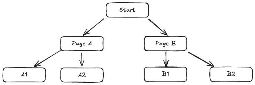
• Root: your starting page.
• Branches: each choice point.
• Levels: how many steps into the story you go.

In model checking, we take a Kripke graph and “unfold” it into a tree of all possible infinite state-sequences, just like showing every playthrough of your adventure game.

Now let’s talk about CTL

CTL lets you ask questions about all or some of those branches, combining:

Path quantifiers

• A (“for All paths”)
• E (“there Exists at least one path”)

Temporal operators

• X f: in the eXt page → f holds
• F f: at some future page → f holds
• G f: on Globally (always) → f holds
• f U g: f holds Until g holds

CTL Form	Meaning (every branch)	Meaning (some branch)
AX f	on All next pages f
EX f		on Exists a next page f
AF f	on all branches, Finally f
EF f		there exists a branch where f eventually happens
AG f	Globally on all branches f
EG f		there exists a branch where f always holds
A[f U g]	on all branches, f holds until g
E[f U g]		exists a branch where f holds until g

Example: In a treasure-hunt game, let treasure mean “you reach the treasure room,” and monster mean “you encounter a monster.”

• AG ¬monster: no matter how you play, you never meet a monster.
• EF treasure: there is at least one way to win the treasure.
• AF treasure: every path eventually leads to treasure (you can’t get stuck).

Question 1 of 8

In the treasure-hunt game, how would you express “on all next moves, you will not encounter a monster”?

AX ¬monsterEX ¬monsterAG ¬monsterEG ¬monster

Semantics of CTL

Let K be your computation tree (all possible game sessions), and s a particular page/state:

• s ⊨ p: Proposition p (a simple fact) is true in page s.
• s ⊨ EX f: There is E one immediate choice from s leading to a page where f holds.
• s ⊨ AX f: On All immediate choices from s, f holds next.
• s ⊨ EF f: There exists E some continuation (branch) from s where f happens Finally.
• s ⊨ AF f: On All continuations, f will happen eventually.
• s ⊨ E[f U g]: There exists a branch where f holds at every step until g becomes true.
• s ⊨ A[f U g]: On all branches, f holds until g does.

Formally these are defined over infinite traces of K.

Question 1 of 7

In the treasure-hunt game, if s ⊨ treasure, what does that mean?

The proposition `treasure` is true in the current pageThere exists a path where you will eventually find the treasureOn all paths you will always have the treasureYou just encountered a monster

Handy Equivalences

CTL has many logical shortcuts—here are a few you’ll use most:

Equivalence	Read as
¬AX f ⇔ EX ¬f	“Not always next f” = “There exists next not-f”
¬AG f ⇔ EF ¬f	“Not always globally f” = “Exists finally not-f”
AF f ⇔ A[⊤ U f]	“Eventually f on all paths” = “true until f”
E[f U g] ⇔ ¬A[¬g U ¬f]	dual of until

Comparing CTL and LTL

1. Linear vs. Branching Time

LTL (Linear‐time Temporal Logic)

Imagine watching a single movie from start to finish—there’s only one storyline. You can make statements like:

• "Eventually, the hero wins."
• "The villain never shows up."

Key idea: Time is a single line of moments.

CTL (Computation‐Tree Logic)

Now think of a choose‐your‐own‐adventure book that branches at each decision point. You can ask questions like:

• "On every possible storyline, the hero never dies."
• "There is some sequence of choices where the hero finds the treasure."

Key idea: Time is a tree of all possible futures.

Everyday Example

• LTL: "In my morning routine, I always brush my teeth eventually."
• CTL:
  • AF brush: No matter which morning‐routine branch I take, I will eventually brush my teeth.
  • EF latte: There’s at least one routine where I eventually get a latte.

---

2. Compositionality: Building Big Systems from Small

A logic is compositional with respect to synchronous product if you can check two pieces separately and then conclude something about the combined system.

• LTL is compositional:

  • If system A satisfies "always safe" and system B satisfies "always responsive," then running A and B together will satisfy "always (safe and responsive)."
  • Formally: If ( K₁ ⊨ f₁ ) and ( K₂ ⊨ f₂ ), then ( (K₁ × K₂) ⊨ (f₁ ∧ f₂) ).

• CTL is not fully compositional:

  • Because CTL can interleave "for all paths" and "there exists a path" in complex ways, you can’t always combine separate guarantees into a joint one without re‐checking the product model.

---

3. Expressive Power: What You Can (and Can’t) Say

CTL and LTL are incomparable—each can express properties the other cannot.

• CTL‐only examples:

  • AX EX p: "On every next step, there exists a further next step where ( p ) holds."
    (You can’t write this in pure LTL.)
  • AF AG p: "Eventually, you reach a point from which ( p ) holds globally on all futures."
    (No equivalent LTL formula exists.)

• LTL‐only examples:

  • G F p ("infinitely often ( p )"): "p occurs again and again forever."
    (There is no CTL formula that forces ( p ) to recur infinitely often on every path without mixing A/E in a way CTL disallows.)

Dropping “A” to See if You Really Need Branching

Given a CTL formula like AFAG p, delete every A (“for All paths”) and see if you get the same meaning. If you do, then your property didn’t truly need branching, it’s just an LTL property in disguise.

Example:

• p = “the door is unlocked.”
• AFAG p says: “On every way you might push or pull, eventually you reach a state from which no matter what, the door stays unlocked forever.”
• Delete the As → you get F G p: “Eventually the door becomes permanently unlocked,” along one sequence of pushes/pulls.

1. Model “push” or “pull” as two choices.
2. Check whether every sequence ends up in a state where all future choices keep it unlocked.
3. If that always matches what happens along one sequence (i.e. F G p), then you didn’t need CTL—you could’ve just used LTL.

Why AFAG p Cannot Become an LTL Formula

Counter-Story: The Two-Lane Road

• You start at a fork. Left lane (Lane 1) loops back to itself forever and has a green light (p). Or you can turn right once into a road (Lane 2 → Lane 3) that then loops green forever.
• Along every infinite drive, eventually you end up on a permanently green road ⇒ F G p holds.
• But is there a point from which all possible next turns stay green? In Lane 1 you can still (at any time) choose to turn right into Lane 2 (where there’s that one blue (¬p) section). So AG p never holds at any point ⇒ AFAG p fails.

You see F G p is true but AFAG p is false—so no LTL formula can capture AFAG p’s extra “all-paths” twist.

Equivalences

CTL	LTL	Read as
AG p	G p	“always p” vs. “globally p”
AF p	F p	“eventually p on all paths”
EX p	(no direct LTL)	“there exists one next state with p”
AX p	X p	“on all next states p holds”
E[f U g]	(f U g)	“there is a path where f until g”
¬AX f ↔ EX ¬f	(duality)	“not all next f” = “there exists next not-f”